Beginner course @ CMD44
Welcome to the STATE hands-on tutorial at CMD44. In the following, how to run the STATE examples for this hands on is desdribed. A documentation of the STATE code can be found here.
Getting started
First of all, we log in to the cluster system (pyxis).
$ ssh -Y [user_name]@pyxis.mp.es.osaka-u.ac.jp
or
$ ssh -Y -l [user_name] pyxis.mp.es.osaka-u.ac.jp
where [user_name] is your user name assigned. If the above commands do not work, use pxyis, instead of pyxis.mp.es.osaka-u.ac.jp.
Then, we are going to set up the STATE program, pseudopotentials, and example files.
This is done by executing the following command in the home directory (${HOME} or ~) as:
$ git clone -b cmd_beginner https://github.com/ikuhamada/state-setup.git STATE
See also my github page.
Then, go to the STATE directory
$ cd STATE
and execute the following
$ ./state-setup.sh
To make sure the command search path is update, type the following
$ source ~/.bashrc
and you are all set!
The source file is located in ${HOME}/STATE/src and examples ${HOME}/STATE/examples.
Go to the STATE directory by typing
$ cd ~/STATE
and
$ ls
you can find the directories as:
examples/ gncpp/ src/
Let us move to ${HOME}/STATE/examples to run the examples.
Carbon monoxide
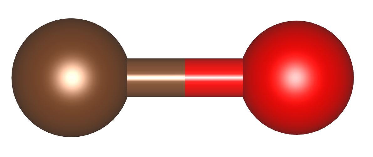
As the first example, let us use the carbon monoxide (CO) molecule in a box.
Go to CO in the examples directory, and have a look at by cat nfinp_scf
WF_OPT    DAV
NTYP      2
NATM      2
GMAX      5.50
GMAXP     20.00
NSCF      200
MIX_ALPHA 0.8
WIDTH     0.0010
EDELTA    1.D-10
NEG       8
CELL      6.00  4.00  4.00  90.00  90.00  90.00
&ATOMIC_SPECIES
 C  12.011  pot.C_pbe1
 O  15.999  pot.O_pbe1
&END
&ATOMIC_COORDINATES
  0.0000  0.0000  0.0000  1  1  1
  2.2000  0.0000  0.0000  1  1  2
&END
Short description of the input variables can be found here
Let us review the job script by cat run.sh
#$ -S /bin/sh
#$ -cwd
#$ -q all.q
#$ -pe smp 4
#$ -N CO

# Disable OPENMP parallelism

export OMP_NUM_THREADS=1

# Set the execuable of the STATE code

ln -fs ${HOME}/STATE/src/state/src/STATE .

# Set the pseudopotential data

ln -fs ../gncpp/pot.C_pbe1
ln -fs ../gncpp/pot.O_pbe1

# Set the input/output file

INPUT_FILE=nfinp_scf
OUTPUT_FILE=nfout_scf

# Run!

mpirun -np $NSLOTS ./STATE < ${INPUT_FILE} > ${OUTPUT_FILE}
and submit!
$ qsub run.sh
The output nfout_scf starts with the header
***********************************************************************
*                                                                     *
*                                                                     *
*                                                                     *
*              ******  ********    **    ******** ********            *
*             ******** ********   ****   ******** ********            *
*             **          **     **  **     **    **                  *
*              ***        **    ********    **    ******              *
*                ***      **   **********   **    ******              *
*                  **     **  **        **  **    **                  *
*             ********    ** **          ** **    ********            *
*              ******     ** VERSION 5.6.14 **    ********            *
*                               RICS-AIST                             *
*                           OSAKA UNIVERSITY                          *
*                                                                     *
***********************************************************************
and at the convergence, total energy, its components, and Fermi energy are printed as
      TOTAL ENERGY AND ITS COMPONENTS
   TOTAL ENERGY     =         -22.21942426 A.U.
 KINETIC ENERGY     =           9.92111450 A.U.
 HARTREE ENERGY     =           5.12121884 A.U.
      XC ENERGY     =          -5.89585659 A.U.
   LOCAL ENERGY     =         -20.23161778 A.U.
NONLOCAL ENERGY     =           6.73686206 A.U.
   EWALD ENERGY     =         -17.87114528 A.U.
      PC ENERGY     =           0.00000000 A.U.
ENTROPIC ENERGY     =           0.00000000 A.U.

                        FERMI ENERGY =       0.43248214
along with the forces acting on atoms
    ATOM              COORDINATES                        FORCES
MD:    1
MD:    1  C   0.000000   0.000000   0.000000   0.01852  0.00000  0.00000
MD:    2  O   2.200000   0.000000   0.000000  -0.01858  0.00000  0.00000
Congratulations! We see the victory cat at the end of the output file:-)
HHHHHHHHHHHHHHHHHHHHHHHHHHHHHHHHHHHHHHHHHHHHHHHHHHHHHHHHHHHHHHHHH
HHHHHHHHHHHHHHHHHHHHHHHHHHHHHHHHHHHHHHHHHHHHHHHHHHHHHHHHHHHHHHHHH
                          _______________________
    __________   _______/______v______v______v___]
   D          | |                                 |
   D   A A    | | Congratulations!                |  C( > < )D
 --  =(^.^)=  | |  The calculation has converged. |    = o =
|     @@@@@   | |                                 |    (    )~
/--=O=-+-=O=---+--=O=--+--==O==--+--==O==--+--=O=-+--=O=---=O=-/

HHHHHHHHHHHHHHHHHHHHHHHHHHHHHHHHHHHHHHHHHHHHHHHHHHHHHHHHHHHHHHHHH
HHHHHHHHHHHHHHHHHHHHHHHHHHHHHHHHHHHHHHHHHHHHHHHHHHHHHHHHHHHHHHHHH
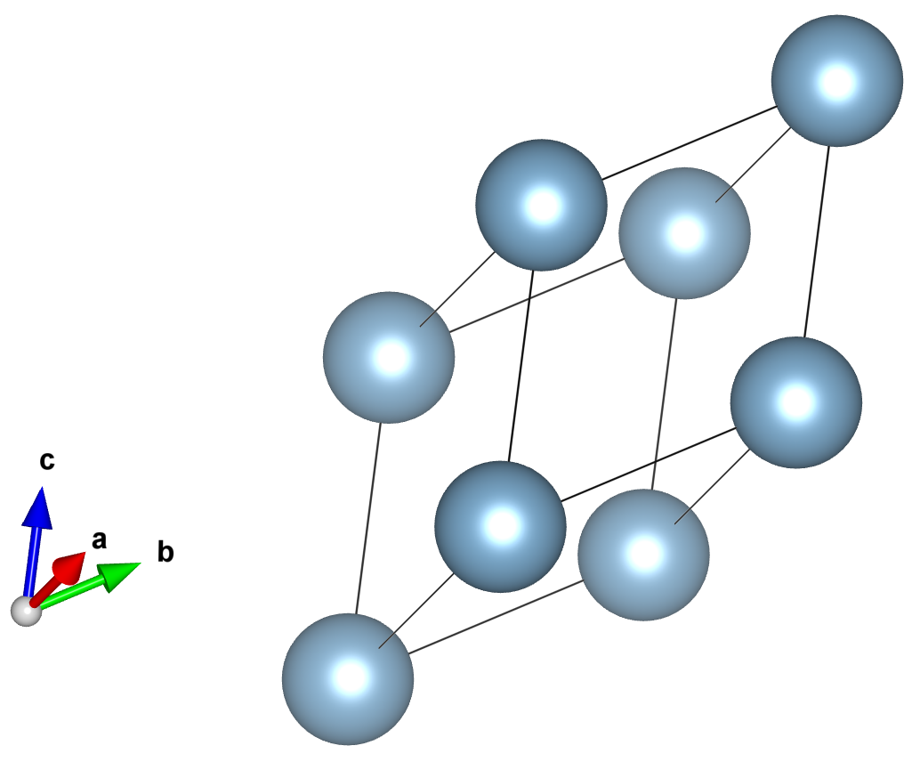
Silicon
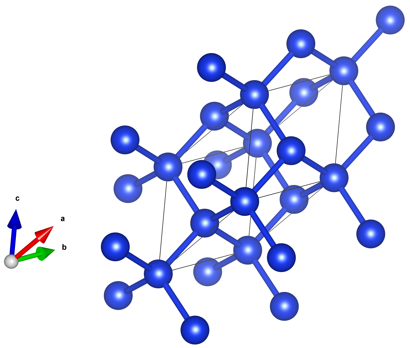
This example explains how to perform a self-consistent field (SCF) calculation and cell (volume) optimization by using a crystalline silicon in the diamond structure as an example.
SCF
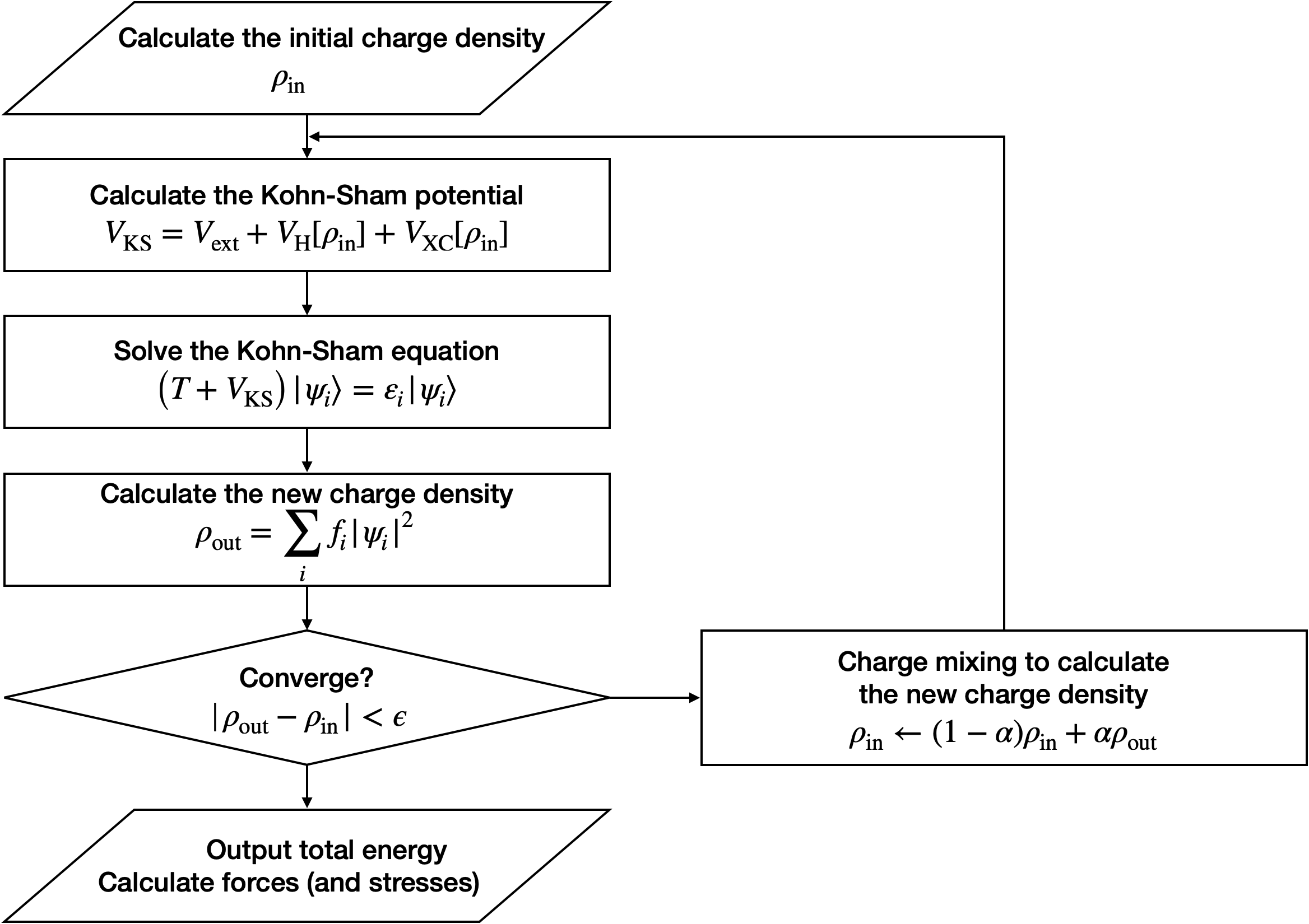
In this example, we are going to learn how to run the SCF calculation. Below is a flowchart for the SCF calculation:
Let us have a look at the input file for the SCF calculation nfinp_scf by typing in the Si directory:
$ cat nfinp_scf
nfinp_scf:
#
# Crystalline silicon in the diamond structure
#
WF_OPT    DAV
NTYP      1
NATM      2
TYPE      2
NSPG      227
GMAX      4.00
GMAXP     8.00
KPOINT_MESH    8   8   8
WIDTH     0.0002
EDELTA    0.5000D-09
NEG    8
CELL   10.30  10.30  10.30  90.00  90.00  90.00
&ATOMIC_SPECIES
 Si 28.0900 pot.Si_pbe1
&END
&ATOMIC_COORDINATES CRYSTAL
      0.000000000000      0.000000000000      0.000000000000    1    1    1
      0.250000000000      0.250000000000      0.250000000000    1    1    1
&END
By default wave function optimization (single-point calculation) is performed (WF_OPT) with the Davidson algorithm (DAV), and structural optimization is not performed (Short description of the input variables can be found here).
Let us review the job script run.sh:
#$ -S /bin/sh
#$ -cwd
#$ -q all.q
#$ -pe smp 4
#$ -N Si

#disable OPENMP parallelism
export OMP_NUM_THREADS=1

# execuable of the STATE code
ln -fs ${HOME}/STATE/src/state/src/STATE .

# pseudopotential data
ln -fs ../gncpp/pot.Si_pbe1

# launch STATE
mpirun -np $NSLOTS ./STATE < nfinp_scf > nfout_scf
By using the above input file and job script, we submit the job as:
$ qsub run.sh
Status of your job can be monitored by using qstat as:
$ qstat
After the calculation is done, check the output file nfout_scf and make sure that lattice vectors and atomic positions are correct.
The primitive lattice vectors are given as:
PRIM. LAT. VECTOR(BOHR) :        0.000000       5.150000       5.150000
PRIM. LAT. VECTOR(BOHR) :        5.150000       0.000000       5.150000
PRIM. LAT. VECTOR(BOHR) :        5.150000       5.150000       0.000000
and atomic positions:
********************************* ATOMS *******************************
  ATOM    X(BOHR)    Y(BOHR)    Z(BOHR)     TAUX    TAUY    TAUZ IW  IR
  1  1    0.00000    0.00000    0.00000   0.0000  0.0000  0.0000  1   0
  2  1    2.57500    2.57500    2.57500   0.2500  0.2500  0.2500  1   0
***********************************************************************
The exchange-correlation (XC) functional used is printed as:
EXCHANGE CORRELATION FUNCTIONALS : ggapbe
and make sure that this is what you want to use.
In this example, we use the generalized gradient approximation (GGA) to the XC functional of Perdew, Burk and Ernzerhof (PBE), which is abreviated as ggapbe in STATE.
The convergence of the total energy can be monitored from the output. It looks like:
***********************************************************************
*                                                                     *
*                              START SCF                              *
*                                                                     *
***********************************************************************

 NSCF NADR            ETOTAL          EDEL          CDEL CONV      TCPU
    1    0       -6.05513096   0.60551E+01   0.32033E-02    0      0.40
    2    1       -7.84013758   0.17850E+01   0.50625E-02    0      0.08
    3    2       -7.87244596   0.32308E-01   0.45624E-02    1      0.08
    4    3       -7.87086756   0.15784E-02   0.76306E-02    1      0.08
    5    4       -7.87352176   0.26542E-02   0.13466E-02    1      0.08
    6    5       -7.87351941   0.23528E-05   0.56367E-03    2      0.08
    7    6       -7.87353730   0.17887E-04   0.40389E-03    2      0.08
    8    7       -7.87355183   0.14538E-04   0.21148E-03    2      0.08
    9    8       -7.87355489   0.30598E-05   0.15435E-03    2      0.08
   10    9       -7.87355832   0.34247E-05   0.95948E-05    3      0.08
   11   10       -7.87355833   0.93097E-08   0.45654E-05    3      0.08
   12   11       -7.87355833   0.29345E-08   0.19696E-05    3      0.08
   13   12       -7.87355833   0.57462E-09   0.17709E-06    4      0.08
   14   13       -7.87355833   0.11322E-10   0.10973E-06    5      0.08
   15   14       -7.87355833   0.90061E-12   0.54074E-07    6      0.08
At the convergence, the total energy and its componets are printed as:
      TOTAL ENERGY AND ITS COMPONENTS
   TOTAL ENERGY     =          -7.87355833 A.U.
 KINETIC ENERGY     =           3.01922419 A.U.
 HARTREE ENERGY     =           0.55014198 A.U.
      XC ENERGY     =          -2.40098652 A.U.
   LOCAL ENERGY     =          -0.84294926 A.U.
NONLOCAL ENERGY     =           0.16885291 A.U.
   EWALD ENERGY     =          -8.36784162 A.U.
      PC ENERGY     =           0.00000000 A.U.
ENTROPIC ENERGY     =           0.00000000 A.U.
NOTE this message is NOT printed when the convergence is not achieved.
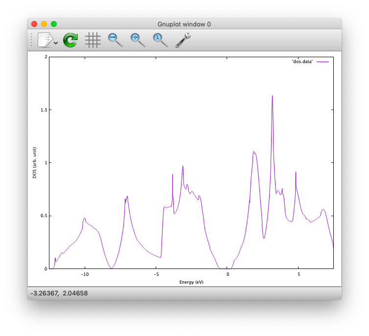
In addition, total density of states (DOS) is printed to dos.data, which can be plotted with, for instantce, gnuplot as
$ gnuplot
gnuplot> set xrange [-12.5:7.5]
gnuplot> set yrange [0:2.0]
gnuplot> set xlabel 'Energy (eV)'
gnuplot> set ylabel 'DOS (arb. unit)'
gnuplot> plot 'dos.data' w l
The resulting DOS looks as follows:
Note
The origin of energy is set to the Fermi level, which is automatically determined even in a gapped system (even in a molecule). For an insulator/semiconductor, it is suggested to set the origin of energy to the valence band maximum. Otherwise the Fermi level should be set at the middle of the band gap.
Cell optimization
In the current version of STATE, the stress tensor is not (yet!) calculated, and the cell optimization should be performed manually.
Let us change the lattice constant from 10.20 Bohr to 10.50 Bohr by 0.05 Bohr by changing the input variable CELL
CELL 10.20 10.20 10.20 90.00 90.00 90.00
CELL 10.25 10.25 10.25 90.00 90.00 90.00
…
CELL 10.50 10.50 10.50 90.00 90.00 90.00
For each lattice constant we prepare an input file as nfinp_scf_10.20, nfinp_scf_10.25, … nfinp_scf_10.50 and submit jobs by changing the input and output files in the job script.
$ qsub run.sh
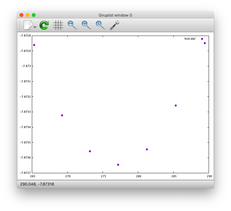
To collect the volume-energy (E-V) data, here we use state2ev.sh script in state-5.6.6/util/ as
$ state2ev.sh nfout_scf_* > etot.dat
This can be visualized by using, for example, gnuplot as
$ gnuplot
gnuplot> plot 'etot.dat' pt 7
The output looks like
Furthermore, by using the eosfit in the util directory as
$ eosfit etot.dat
one can see the following
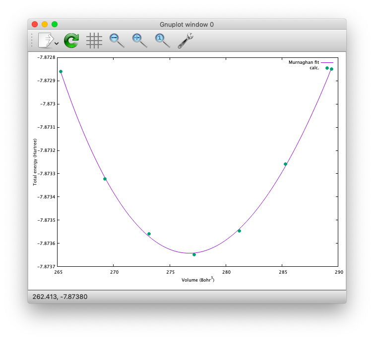
and the equilibrium volume is obitained.
The equilibrium volume (v0), energy (e0), bulk modulus (b0), and derivative of bulk modulus (b0’) can be found in eosfit.param.
The resulting equilibrium lattice constant is 10.3455 Bohr (5.475 Angstrom).
Compare with experimental and theoretical values in the literature.
Question
How to derive the equilibrium lattice constant from the volume?
How good/bad is the equilibrium lattice constant obtained here?
Further exercise
In the current working directory, you can find subdirectory LDAPW91, which contains the input files and job scripts for the calculations using the local density approximation (LDA). Calculate the equilibrium lattice constant and compare it with that obtained using PBE (above) and experimental value. There is also another subdirectory PBEsol for another GGA XC functional. Calculate the equilibrium lattice constant using the PBEsol XC functional and compare the accuracies of the theoretical values.
Aluminum
In this example, how to deal with a metallic system with the smearing method is briefly described by using the crystalline aluminium in the face centered cubic (fcc) structure.
SCF
In the Al directory, we use the following input file for the SCF calculation.
nfinp_scf:
#
# Crystalline aluminum in the face centered cubic structure
#
WF_OPT  DAV
NTYP    1
NATM    1
TYPE    2
NSPG    221
GMAX    4.00
GMAXP   8.00
KPOINT_MESH   12  12  12
SMEARING MP
WIDTH   0.0020
EDELTA  0.5000D-09
NEG     6
CELL    7.50000000   7.50000000   7.50000000  90.00000000  90.00000000  90.00000000
&ATOMIC_SPECIES
Al 26.9815386 pot.Al_pbe1
&END
&ATOMIC_COORDINATES CRYSTAL
      0.000000000000      0.000000000000      0.000000000000    1    0    1
&END
Here we set the smearing function of Methefessel and Paxton (MP) as
SMEARING MP
and smearing width
WIDTH 0.0020
We can also use negative WIDTH without specifying SMEARING to enable the smearing function.
In this case the MP smearing function is automatically set.
See the manual for the available smearing functions.
Submit the STATE job as
$ qsub run.sh
After the convergence, let us plot DOS printed in dos.data as in the case of Si using gnuplot:
$ gnuplot
gnuplot> set xrange [-12.5:7.5]
gnuplot> set yrange [0.0:0.4]
gnuplot> set xlabel 'Energy (eV)'
gnuplot> set ylabel 'DOS (arb. unit)'
gnuplot> plot 'dos.data' w l
The resulting DOS looks as follows:
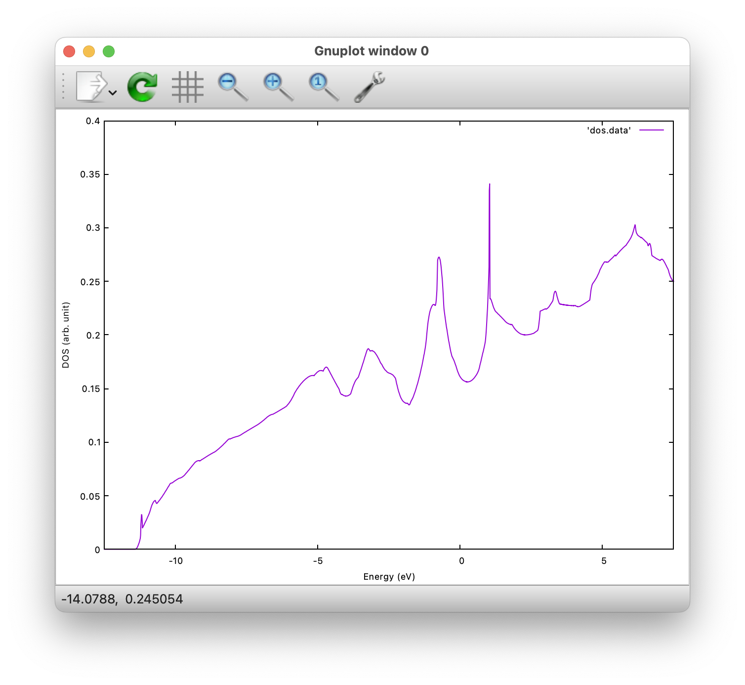
We can see that we obtained the free-electron-like DOS and that there is not band gap around the Fermi level in contrast to Si.
Note
Total energy of the metallic system is sensitive to the smearing function and width, and the number of k-points, and they should be determined very carefully before the production run. Detail is discussed in the tutorial (to be completed).
Nickel
This example shows how to perform a calculation of a spin-polarized system using the ferromagnetic Ni in the fcc structure.
The directory is Ni.
SCF and DOS
Input file (
nfinp_scf)
#
# Ferromagnetic Ni in the fcc structure
#
WF_OPT DAV
NTYP   1
NATM   1
TYPE   2
NSPG   221
GMAX    5.00
GMAXP  15.00
KPOINT_MESH   12  12  12
MIX_ALPHA 0.3
SMEARING MP
WIDTH  0.0020
EDELTA 0.5000D-09
NSPIN  2
NBZTYP 102
NEG    10
CELL   6.70  6.70  6.70  90.00  90.00  90.00
&ATOMIC_SPECIES
 Ni 58.6900 pot.Ni_pbe4
&END
&INITIAL_ZETA
 0.20
&END
&ATOMIC_COORDINATES CRYSTAL
      0.000000000000      0.000000000000      0.000000000000    1    1    1
&END
To allow the spin polarized calculation, one has to set
NSPIN 2
along with the initial magnetization as
&INITIAL_ZETA
 0.20
&END
for each atomic species.
Submitting a job:
$ qsub run.sh
As above, dos.data is automatically generated. In the case of spin polarized system, the first column of dos.data contains energy, second and third columns contain DOS for spin up and down respectively.
This can be plotted by using gnuplot as follows:
$ gnuplot
gnuplot> set xrange [-10:5]
gnuplot> set yrange [0:4]
gnuplot> set xlabel 'E-E_F (eV)'
gnuplot> set ylabel 'DOS (state/eV)'
gnuplot> plot 'dos.data' using ($1):($2) w l title 'Spin-up','dos.data' using ($1):($3) w l title 'Spin-down'
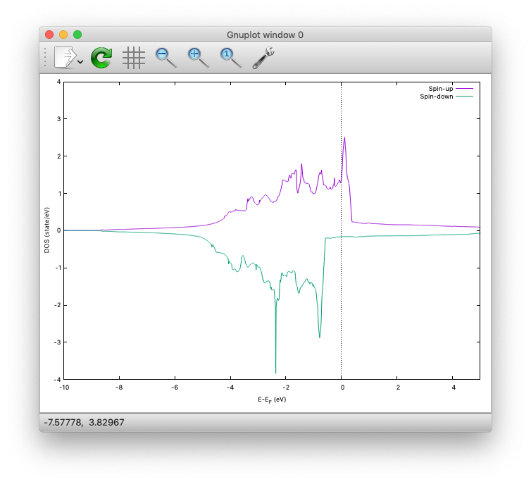
The spin-polarized DOS looks like:

Or by using the following:
gnuplot> set xrange [-10:5]
gnuplot> set yrange [-4:4]
gnuplot> set yzeroaxis
gnuplot> set xlabel 'E-E_F (eV)'
gnuplot> set ylabel 'DOS (state/eV)'
gnuplot> plot 'dos.data' using ($1):($2) w l title 'Spin-up','dos.data' using ($1):(-$3) w l title 'Spin-down'
One may obtain the spin-polarized DOS like:
Question
Compare DOS obtained using the pseudopotential method (present) with that using the all-electron one (e.g., FLAPW and KKR).
Iron
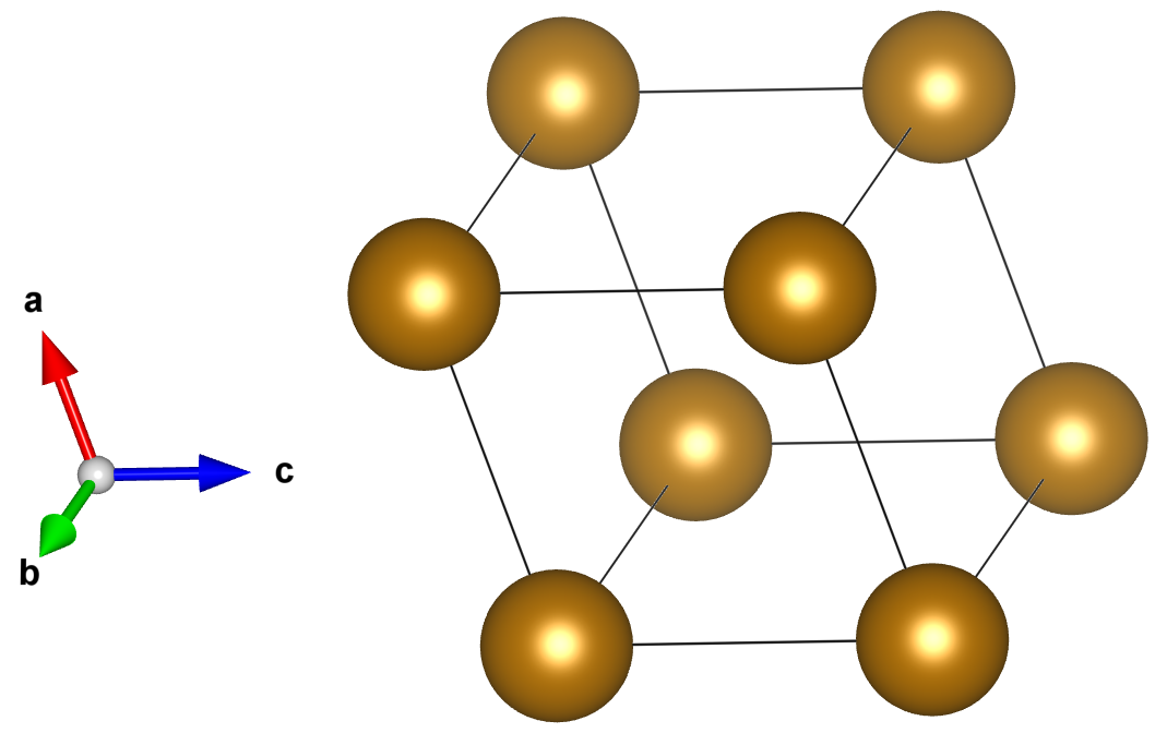
This is yet another example to show how to perform a calculation of a spin-polarized system using the ferromagnetic Fe in the bcc structure.
The directory is Fe.
SCF
Input file (
nfinp_scf)
#
# Fe in the bcc structure
#
WF_OPT      DAV
NTYP        1
NATM        1
TYPE        1
NSPG        229
GMAX        5.00
GMAXP       15.00
KPOINT_MESH 08 08 08
MIX_ALPHA   0.50
BZINT       TETRA
EDELTA      1.0D-10
NSPIN       2
NEG         16
XCTYPE      ggapbe
CELL  5.40461887  5.40461887  5.40461887  90.00000000  90.00000000  90.00000000
&ATOMIC_SPECIES
 Fe  55.845000 pot.Fe_pbe3
&END
&INITIAL_ZETA
  0.2000
&END
&ATOMIC_COORDINATES CRYSTAL
      0.000000000000      0.000000000000      0.000000000000    1    0    1
&END
In this case, we use the tetrahedron method for the Brillouin zone integration.
Make sure if the input and output files are propley given in the job script (run.sh), submit a job by:
$ qsub run.sh
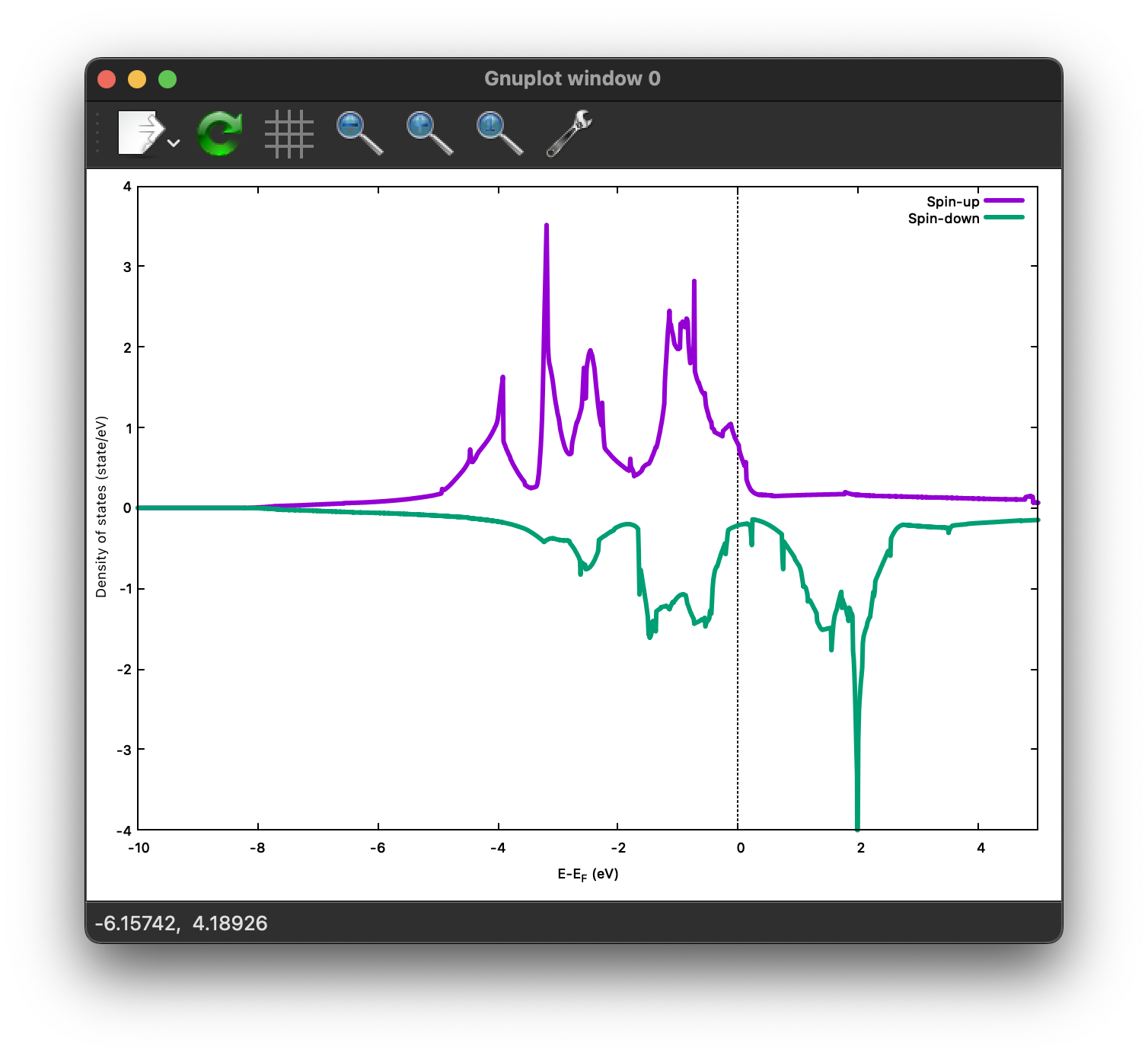
As in the case of the Ni example, let us plot the density of states using gnuplot as follows
gnuplot> set xrange [-10:5]
gnuplot> set yrange [-4.0:4.0]
gnuplot> set xlabel 'E-E_F (eV)'
gnuplot> set ylabel 'Density of states (state/eV)'
gnuplot> plot 'dos.data' using ($1):($3) title 'Spin-up' with lines lt 1 lw 3,'' using ($1):(-$2) title 'Spin-down' with lines lt 2 lw 3
Then you may obtain DOS as shown in the following figure:
Question
How do you compare DOS from the plane-wave pseudopotential calculation with that from all-electron methods such as KKR and FLAPW?
To improve the accuracy of DOS, we can increase the number of k-points without performing a new SCF calculation with denser k-point grid, by performing a non-SCF calculation using the converged electron density. This can be done by adding a key word TASK NSCF in the input file as:
Non-SCF and DOS
Input file (
nfinp_nscf)
#
# Fe in the bcc structure
#
TASK        NSCF
WF_OPT      DAV
NTYP        1
NATM        1
TYPE        1
NSPG        229
GMAX        5.00
GMAXP       15.00
KPOINT_MESH 16 16 16
MIX_ALPHA   0.50
BZINT       TETRA
EDELTA      1.0D-10
NSPIN       2
NEG         16
XCTYPE      ggapbe
CELL  5.40461887  5.40461887  5.40461887  90.00000000  90.00000000  90.00000000
&ATOMIC_SPECIES
 Fe  55.845000 pot.Fe_pbe3
&END
&INITIAL_ZETA
  0.2000
&END
&ATOMIC_COORDINATES CRYSTAL
      0.000000000000      0.000000000000      0.000000000000    1    0    1
&END
We can see that we are going to use 16 x 16 x 16 k-point mesh in this calculation. Before performing Non-SCF calculation, let us rename dos.data dos.data_08x08x08, and edit the job script and change the input and output file names nfinp_nscf and nfout_nscf, respectively, and submit the job:
$ qsub run.sh
After the calculation, we plot DOS and may obtain the following:
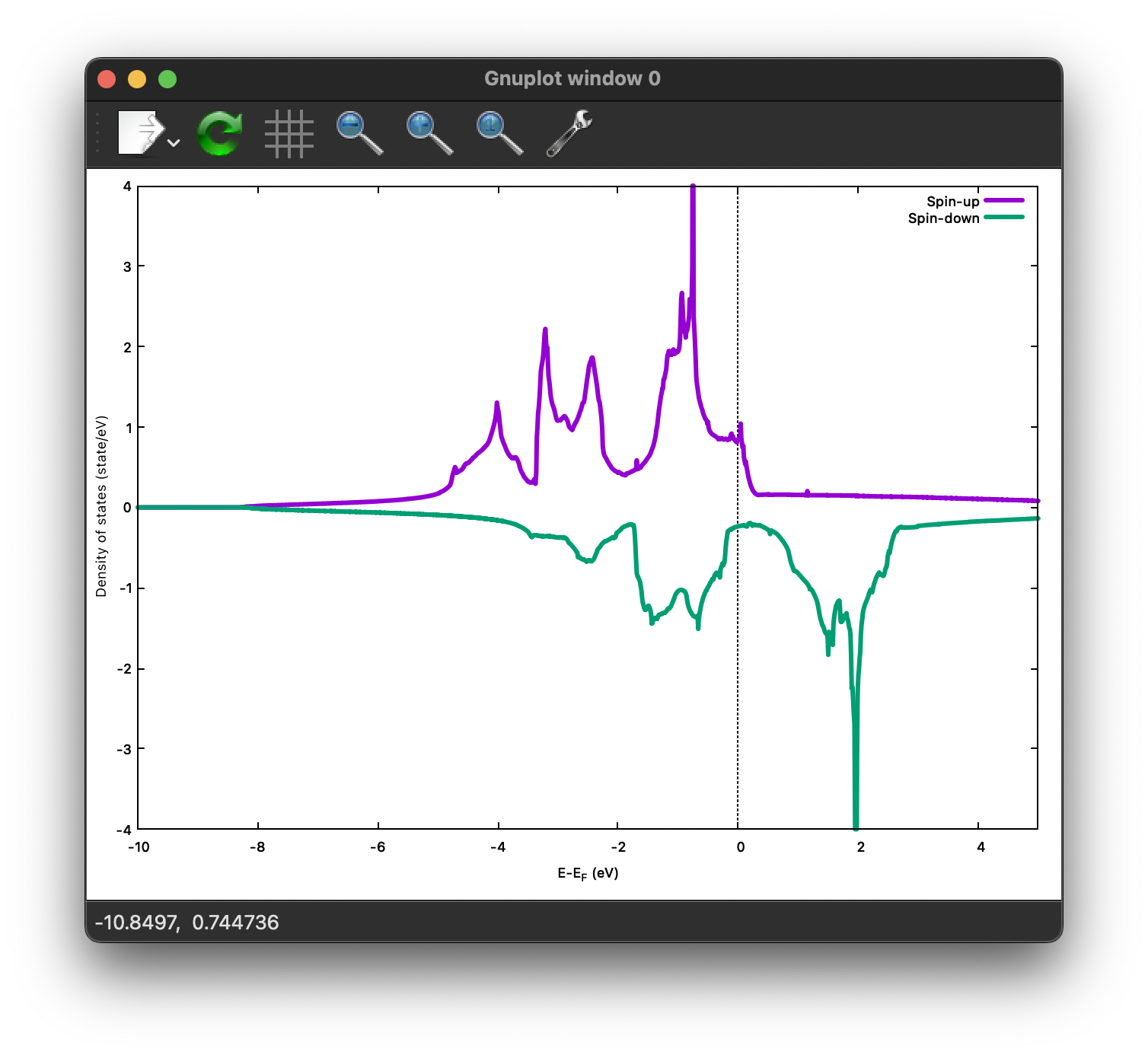
How about the comparison with the all-electron (e.g., FLAPW and KKR) results?
Ethylene
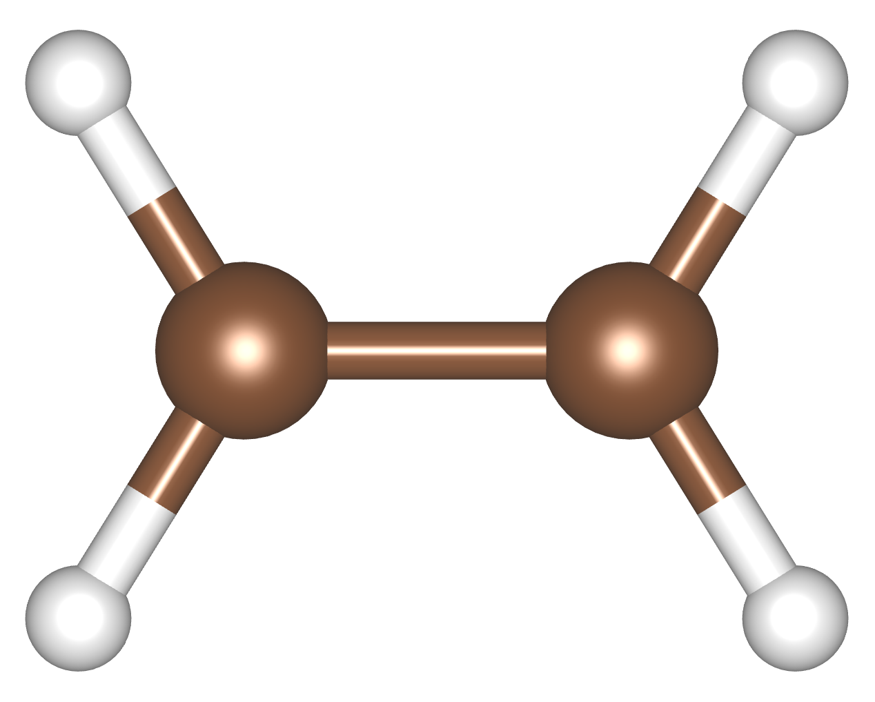
Directory:
C2H4
This example explains how to perform:
geometry optimization
vibrational analysis
molecular dynamics simulation
Geometry optimization
Input file
nfinp_gdiis
#
# Ethylene molecule in a box: geometry optimization with the GDIIS method
#
WF_OPT  DAV
GEO_OPT GDIIS
NTYP   2
NATM   6
TYPE   0
GMAX    5.00
GMAXP  15.00
MIX_ALPHA 0.8
WIDTH   0.0010
EDELTA  0.1000D-08
NEG     10
FMAX    0.5000D-03
CELL   12.00  12.00  12.00  90.00  90.00  90.00
&ATOMIC_SPECIES
 C  12.0107  pot.C_pbe3
 H   1.0079  pot.H_lda3
&END
&ATOMIC_COORDINATES CARTESIAN
      1.262722983300      0.000000000000      0.000000000000    1    1    1
      2.348328846800      1.753458668500      0.000000000000    1    1    2
      2.348328846800     -1.753458668500      0.000000000000    1    1    2
     -1.262722983300      0.000000000000      0.000000000000    1    1    1
     -2.348328846800      1.753458668500      0.000000000000    1    1    2
     -2.348328846800     -1.753458668500      0.000000000000    1    1    2
&END
The keyword GEO_OPT is used to activate the geometry optimization.
In this example, GDIIS algorithm is employed as:
GEO_OPT GDIIS
The force threshold for the geometry optimization is set by the keyword FMAX as:
FMAX 0.5000D-03
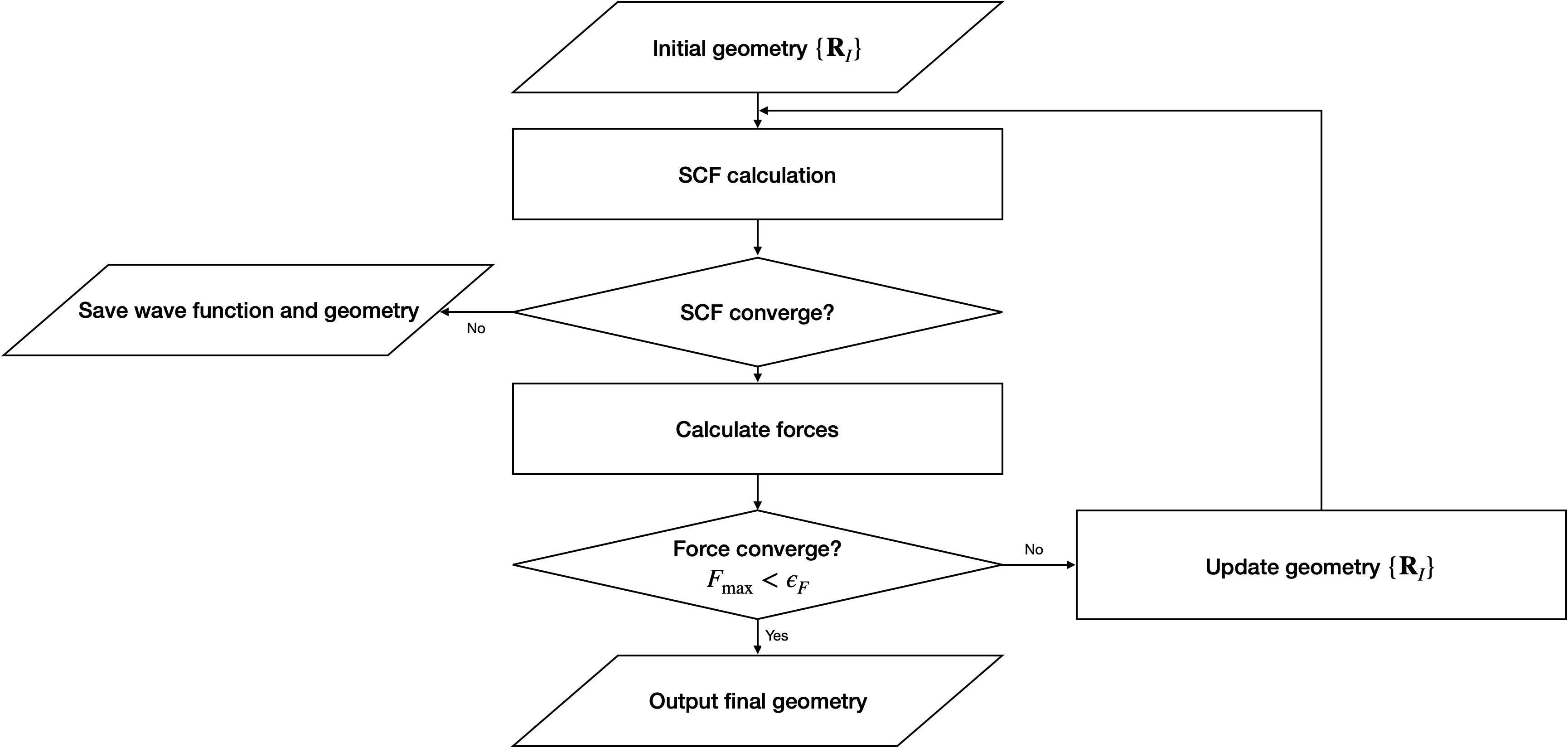
Below is a flowchart for the geometry optimization:
Let us submit the job as:
$ qsub run_gdiis.sh
The convergence of the forces can be monitored by:
$ grep -A1 f_max nfout_gdiis
The result looks like:
   NIT     TotalEnergy     f_max     f_rms      edel      vdel      fdel
     1    -13.90231646  0.001396  0.001303  0.13D-08  0.59D-07  0.13D-08
--
   NIT     TotalEnergy     f_max     f_rms      edel      vdel      fdel
     2    -13.90232125  0.001296  0.001109  0.45D-09  0.47D-07  0.45D-09
--
   NIT     TotalEnergy     f_max     f_rms      edel      vdel      fdel
     3    -13.90233075  0.000965  0.000788  0.27D-09  0.13D-06  0.27D-09
--
   NIT     TotalEnergy     f_max     f_rms      edel      vdel      fdel
     4    -13.90234041  0.000562  0.000459  0.17D-08  0.25D-06  0.17D-08
--
   NIT     TotalEnergy     f_max     f_rms      edel      vdel      fdel
     5    -13.90234848  0.000329  0.000271  0.11D-09  0.91D-07  0.11D-09
Final atomic coordinates in the cartesian coordinate and forces acting on atoms are given as:
                       CONVERGED ENERGY AND FORCES
   NIT     TotalEnergy     f_max     f_rms      edel      vdel      fdel
     5    -13.90234843  0.000349  0.000281  0.25D-09  0.12D-06  0.25D-09

    ATOM              COORDINATES                        FORCES
MD:    5
MD:    1  C   1.260786   0.000001  -0.000000  -0.00035 -0.00000  0.00000
MD:    2  H   2.337963   1.755204  -0.000000  -0.00019 -0.00015  0.00000
MD:    3  H   2.337964  -1.755205  -0.000000  -0.00019  0.00015  0.00000
MD:    4  C  -1.260786   0.000000  -0.000000   0.00035 -0.00000  0.00000
MD:    5  H  -2.337963   1.755204   0.000000   0.00019 -0.00015 -0.00000
MD:    6  H  -2.337963  -1.755204   0.000000   0.00019  0.00015 -0.00000

 EXITING ATOM LOOP
Because the maximum force f_max is smaller than the threshold, the calculation stops with the message:
EXITING ATOM LOOP
The latest geometry is stored in the GEOMETRY file (text file), and in the case of GDIIS, past geometries are stored in gdiis.data.
It is suggested that gdiis.data be deleted or renamed when the number of optimization steps is close to the number of degrees of freedom.
If the structural optimization is not finished, add the keyword RESTART in the input file and submit the job again. To restart the calculation, make sure restart.data file exists in the working directory.
Vibrational analyis
Having obtained the optimized geometry, let us perform the vibrational (normal) mode analysis. This can be done in the following steps.
Frist, we need to create an input file with the optimized geometry.
This can be done by using a utility geom2nfinp as
$ geom2nfinp -i nfinp_gdiis -g GEOMETRY -o nfinp_relaxed
where input parameters from nfinp_gdiis and atomic positions from GEOMETRY are used to create a new input file nfinp_relaxed.
geom2nfinp can also be used to generate an XYZ/XSF file from the optimized geometry.
Type geom2nfinp -h for the usage of the command.
Then we copy nfinp_relaxed to nfinp_vib which looks like:
#
# Ethylene molecule in a box: geometry optimization with the GDIIS method
#
TASK   VIB
WF_OPT DAV
NTYP   2
NATM   6
TYPE   0
GMAX    5.00
GMAXP  15.00
MIX_ALPHA 0.8
WIDTH   0.0010
EDELTA  0.1000D-08
NEG     10
FMAX    0.5000D-03
CELL   12.00  12.00  12.00  90.00  90.00  90.00
&ATOMIC_SPECIES
 C  12.0107  pot.C_pbe3
 H   1.0079  pot.H_lda3
&END
&ATOMIC_COORDINATES CARTESIAN
      1.260767348060     -0.000000889176      0.000000061206    1    1    1
      2.337934105040      1.755199776368      0.000000035554    1    1    2
      2.337933682371     -1.755198581491      0.000000037135    1    1    2
     -1.260766004354     -0.000000071340      0.000000050715    1    1    1
     -2.337933757669      1.755199342527      0.000000064907    1    1    2
     -2.337933482763     -1.755199042963      0.000000067944    1    1    2
&END
We can see the new keyword TASK VIB, which enables one to perform the vibrational analysis.
Note
Make sure the atomic masses in the input file are those you want to use as in some cases we use artificially large/small atomic masses for efficient structural optimization.
In addition to the input file, we need prepare nfvibrate.data as:
1  0.10D+01   1
 1   0.0100000000   0.0000000000   0.0000000000
1 -0.10D+01   1
 1   0.0100000000   0.0000000000   0.0000000000
1  0.10D+01   2
 1   0.0000000000   0.0100000000   0.0000000000
1 -0.10D+01   2
 1   0.0000000000   0.0100000000   0.0000000000
1  0.10D+01   3
 1   0.0000000000   0.0000000000   0.0100000000
1 -0.10D+01   3
 1   0.0000000000   0.0000000000   0.0100000000
...
1  0.10D+01  16
 6   0.0100000000   0.0000000000   0.0000000000
1 -0.10D+01  16
 6   0.0100000000   0.0000000000   0.0000000000
1  0.10D+01  17
 6   0.0000000000   0.0100000000   0.0000000000
1 -0.10D+01  17
 6   0.0000000000   0.0100000000   0.0000000000
1  0.10D+01  18
 6   0.0000000000   0.0000000000   0.0100000000
1 -0.10D+01  18
 6   0.0000000000   0.0000000000   0.0100000000
In the present example, the file contains 2 x 2 x 6 x 3 = 72 lines, which define the atomic displacement in the cartesian coordinate. This is 36 set of displacement composed of 2 lines (in this case). Here I use first two lines as an example:
First line
1 0.10D+01 1
First column : number of displacement(s)
Second column : factor for the displacement
Thrid column : dummy
Second line
1 0.0100000000 0.0000000000 0.0000000000
First column in the second line: the index for the atom displaced
Second-Fourth column in the second line: atomic displacement in the cartesian coordinate.
Actual atomic displacements are atomic displacement (2-4th column in the second line multiplied by the factor).
Submit the job
$ qsub run_vib.sh
and we get nfforce.data in addition to the standard output files, which contains displaced atomic positions and forces acting on atoms, which can be used to calculate the vibrational frequencies.
Then to calculate the dynamical matrix and vibrational frequencies, we use the gif program as follows:
$ gif -f nfforce.data
and we can see the vibrational frequncies printed in the standard output as:
            =========
             SUMMARY
            =========

MODE  WR       : NU(meV)  NU(cm-1)
   1 -0.42D-03 :   12.97    104.63
   2 -0.19D-03 :    8.76     70.63
   3 -0.61D-04 :    4.97     40.06
   4 -0.18D-04 :    2.67     21.50
   5  0.30D-04 :    3.46     27.93
   6  0.28D-03 :   10.71     86.35
   7  0.25D-01 :  100.48    810.43
   8  0.32D-01 :  114.17    920.88
   9  0.34D-01 :  116.25    937.60
  10  0.41D-01 :  128.26   1034.48
  11  0.55D-01 :  148.39   1196.82
  12  0.68D-01 :  165.42   1334.18
  13  0.76D-01 :  175.51   1415.54
  14  0.10D+00 :  201.49   1625.12
  15  0.36D+00 :  379.55   3061.29
  16  0.36D+00 :  381.80   3079.41
  17  0.37D+00 :  388.22   3131.17
  18  0.38D+00 :  393.55   3174.18
The first column, the number of mode, the second column, square of the vibrational frequency in Hartree, and third and fourth columns are vibrational frequencies in meV and wavenumber (cm^-1), respectively.
Warning
New data are always appended to the exsiting nfforce.data. Rename it when (a set of) calculations are finished.
Finally, we visualize the vibrational mode by using the gif2xsf utility.
To use gif2xsf we prepare an XSF, which can be created by using the chkinpf utility as:
$ chkinpf --atom nfinp_vib
By this we are able to create an XSF file for molecule (not periodic boundary condition). Then type
$ gif2xsf -s --xsf C2H4 --gif vib.data --prefix vib
Use C2H4.xsf for the XSF file, vib.data for VIB file, and vib for prefix, and we get separate vib_*.xsf, which can be visualized by using XCrySden or VESTA.
Finite temperature molecular dynamics
In this example, we are going to perform a finite temperature molecular dynamics (MD) simulation.
Input file
nfinp_nhc
#
# Ethylene molecule in a box: finite temperature molecular dynamics
#
WF_OPT  DAV
ION_DYN FTMD
NTYP   2
NATM   6
TYPE   0
GMAX    5.00
GMAXP  15.00
MIX_ALPHA 0.8
WIDTH   0.0010
EDELTA  0.1000D-08
NEG     10
TEMP_CONTROL NHC
TEMPW   300.0D0
WNOSEP  500.0D0
NHC     8
NOSY    15
NDRT    1
CELL   12.00  12.00  12.00  90.00  90.00  90.00
&ATOMIC_SPECIES
 C  12.0107  pot.C_pbe3
 H   1.0079  pot.H_lda3
&END
&ATOMIC_COORDINATES CARTESIAN
      1.262722983300      0.000000000000      0.000000000000    1 1001    1
      2.348328846800      1.753458668500      0.000000000000    1 1001    2
      2.348328846800     -1.753458668500      0.000000000000    1 1001    2
     -1.262722983300      0.000000000000      0.000000000000    1 1001    1
     -2.348328846800      1.753458668500      0.000000000000    1 1001    2
     -2.348328846800     -1.753458668500      0.000000000000    1 1001    2
&END
To perform a molecular dynamics simulation, we set ION_DYN FTMD and how to control the temperature is given as:
TEMP_CONTROL NHC
TEMPW   300.0D0
WNOSEP  500.0D0
NHC     8
NOSY    15
NDRT    1
See the manual for the detailed descriptions on these parameters.
Submit the job
$ qsub run_nhc.sh
In this example, we perform 200 MD steps (default value).
When the calculation is terminated, we get TRAJECTORY containing the trajectory and ENERGIES containing information on temperature and energies.
To visualize the trajectroy, first we need GEOMETRY.xyz, which can be generated by
$ chkinpf --xyz nfinp_nhc -o GEOMETRY.xyz
Then use traj2xyz.pl in the current example directry as
$ ./traj2xyz.pl > traj.xyz
to save the trajectory in the XYZ format.
Use XCrySDen, VMD, or other your favorite visualization software to visualize it (VESTA cannot be used for movies). Here is an example how to use a web-based tool to visualize the molecular dynamics.
Note
Generally, long time molecular dynamics simulation is required to obtain reliable statistical ensemble/average, which cannot be possible within the given hours. In STATE, use CPUMAX to dump the latest geometry and wave functions before the time limit, and restart by using the RESTART keyword. It is also possible to terminate the job by writing a positive number in the nfstop.data.
Cl on Al(100)
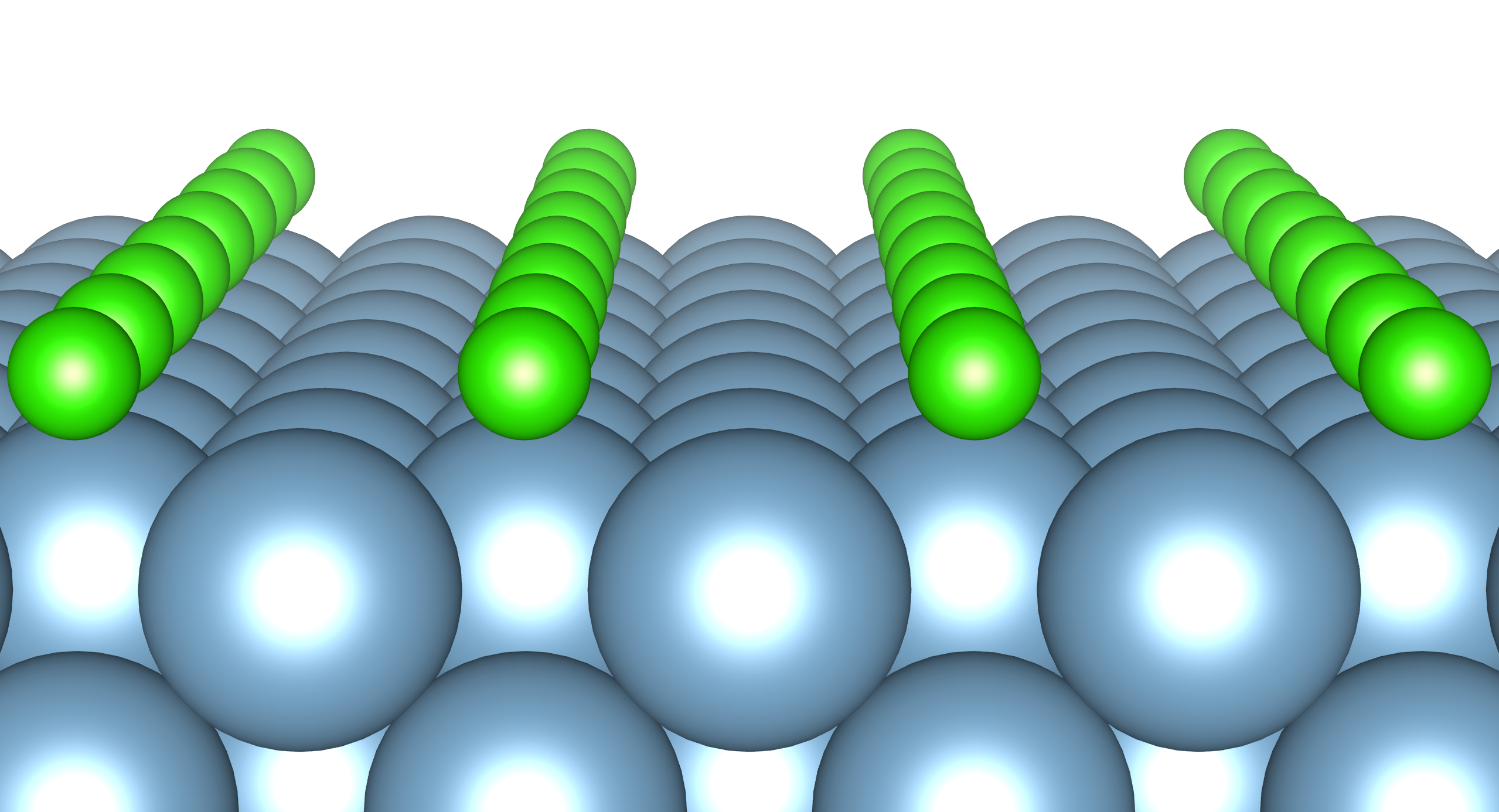
This example explains how to model the surface with an adsobate by using an Al(100) surface with a Cl atom. We also discuss how the periodic boundary condition (PBC) affects the potential (and thus the energy and forces) and how to address the issue by using the effective screening medium (ESM) method.
Geometry optimization with PBC
Go to ClonAl100 and use the following input file (nfinp_gdiis_pbc):
#
# Cl on Al(100)
#
WF_OPT  DAV
GEO_OPT GDIIS
NTYP    2
NATM    7
NSPG    1
GMAX    4.00
GMAXP  10.00
KPOINT_MESH    4   4   1
KPOINT_SHIFT   ON  ON  OFF
SMEARING  MP
WIDTH     0.0020
NEG       16
MIX       BROYDEN2
MIX_ALPHA 0.80
EDELTA   1.000D-09
DTIO     600.00
FMAX     1.000D-03
&ATOMIC_SPECIES
 Al  26.9815 pot.Al_pbe1
 Cl  35.4527 pot.Cl_pbe1
&END
&CELL
      7.653400000000      0.000000000000      0.000000000000
      0.000000000000      7.653000000000      0.000000000000
      0.000000000000      0.000000000000     30.613600000000
&END
&ATOMIC_COORDINATES CARTESIAN
      0.000000000000      0.000000000000      3.700000000000    1    1    2
      0.000000000000      3.826700000000      0.000000000000    1    1    1
      3.826700000000      0.000000000000      0.000000000000    1    1    1
      0.000000000000      0.000000000000     -3.826700000000    1    0    1
      3.826700000000      3.826700000000     -3.826700000000    1    0    1
      0.000000000000      3.826700000000     -7.653400000000    1    0    1
      3.826700000000      0.000000000000     -7.653400000000    1    0    1
&END
We see that how to define the lattice vectors differs from the previous examples.
Subit the STATE job by executing:
$ qsub run.sh
and we get GEOMETRY and gdiis.data in addition to the standard output files.
Warning
When the geometry optimization is performed with the GDIIS method from scratch, make sure that there is no existing gdiis.dta. Furthermore, when the number of optimization steps exceeds the number of degrees of freedom, delete or rename gdiis.data.
Geometry optimization with the ESM method
We then use nfinp_gdiis_esm for the structural optimization with the effective screening medium method, which looks like:
#
# Cl on Al(100)
#
WF_OPT  DAV
GEO_OPT GDIIS
NTYP    2
NATM    7
NSPG    1
GMAX    4.00
GMAXP  10.00
KPOINT_MESH    4   4   1
KPOINT_SHIFT   ON  ON  OFF
SMEARING  MP
WIDTH     0.0020
NEG       16
MIX       BROYDEN2
MIX_ALPHA 0.80
EDELTA   1.000D-09
DTIO     600.00
FMAX     1.000D-03
&ESM
 BOUNDARY_CONDITION BARE
&END
&ATOMIC_SPECIES
 Al  26.9815 pot.Al_pbe1
 Cl  35.4527 pot.Cl_pbe1
&END
&CELL
      7.653400000000      0.000000000000      0.000000000000
      0.000000000000      7.653000000000      0.000000000000
      0.000000000000      0.000000000000     30.613600000000
&END
&ATOMIC_COORDINATES CARTESIAN
      0.000000000000      0.000000000000      3.700000000000    1    1    2
      0.000000000000      3.826700000000      0.000000000000    1    1    1
      3.826700000000      0.000000000000      0.000000000000    1    1    1
      0.000000000000      0.000000000000     -3.826700000000    1    0    1
      3.826700000000      3.826700000000     -3.826700000000    1    0    1
      0.000000000000      3.826700000000     -7.653400000000    1    0    1
      3.826700000000      0.000000000000     -7.653400000000    1    0    1
&END
Diffence from the previous calculation is
&ESM
 BOUNDARY_CONDITION BARE
&END
This enables the ESM calculation. In this case open boundary condition in the surface normal direction is used.
Analysis of the effective and electrostatic potentials
Here we analyze the potentials from PBC and ESM calculations.
Use state2chgpro.sh utility to extract planar average of charge, effective (Kohn-Sham) and electrostatic potentials as:
$ state2chgpro.sh nfout_gdiis_pbc > chgpro.dat_pbc
chgpro.dat_pbc may look like following:
#
# Fermi energy =       -0.05368332 Hartree
#
#          z           Charge             VlHxc               VlH
     0.0000      0.0244720791     -0.5159539900     -0.1911502410
     0.3061      0.0234616356     -0.5090777191     -0.1881052797
     0.6123      0.0227510319     -0.4956732447     -0.1748120165
     0.9184      0.0226562465     -0.4739551828     -0.1543648253
     ...
Here, the first column is the z-coordinate in the Bohr radius, and second, third, and fourth column are the planer averages of charge density, local potential (sum of local pseudo-, Hartree, and XC potentials), and hartree potential, respectively.
By plotting the first (z-coordinate) and third (local potential) colums, and first (z-coordinate) and fourth (electrostatic potential) colums, we get the following potential profile:
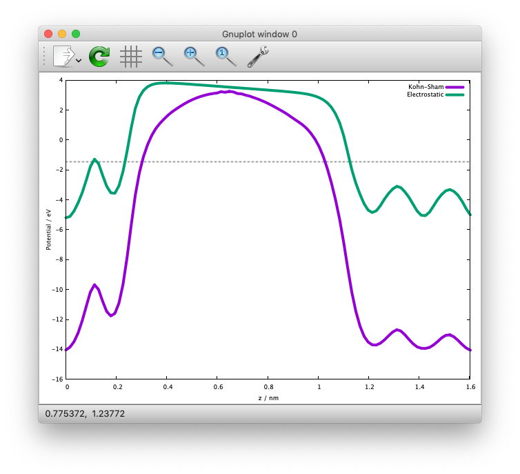
We can see that the electric field is applied to the slab because of the periodic boundary condition.
We also extract the planar average of chargen and potential from the ESM calculations as:
$ state2chgpro.sh nfout_gdiis_esm > chgpro.dat_esm
and we get the following:
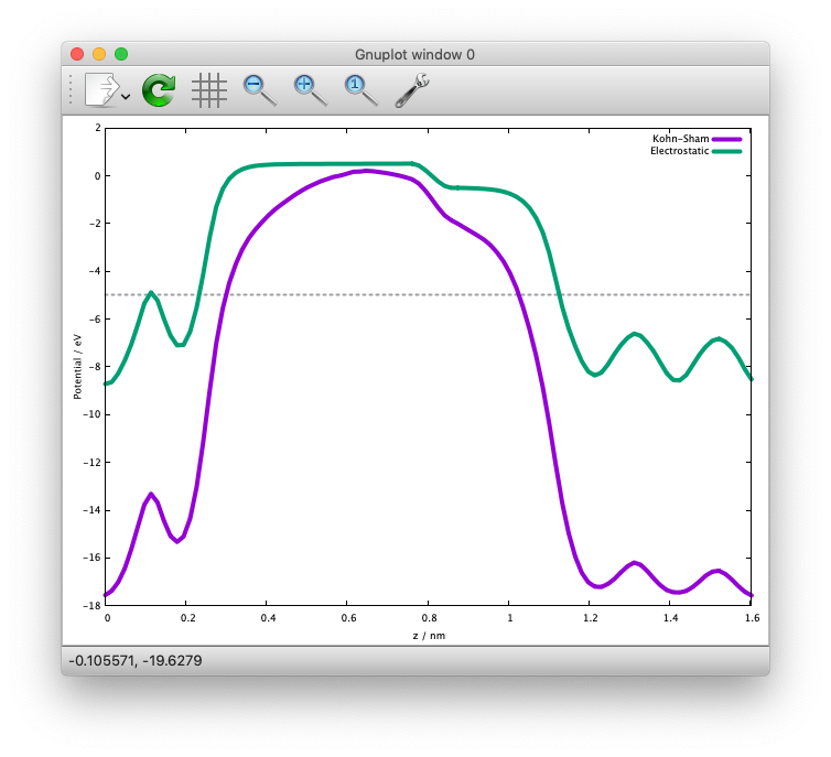
We can see that the potentials are flat in the vacuum region. Mind that the slab is locased near the origin (z=0). The discontinuity is by the plotting reason (actually they are disconnected because we do not use the periodic boundary condition with the ESM method).
Graphene
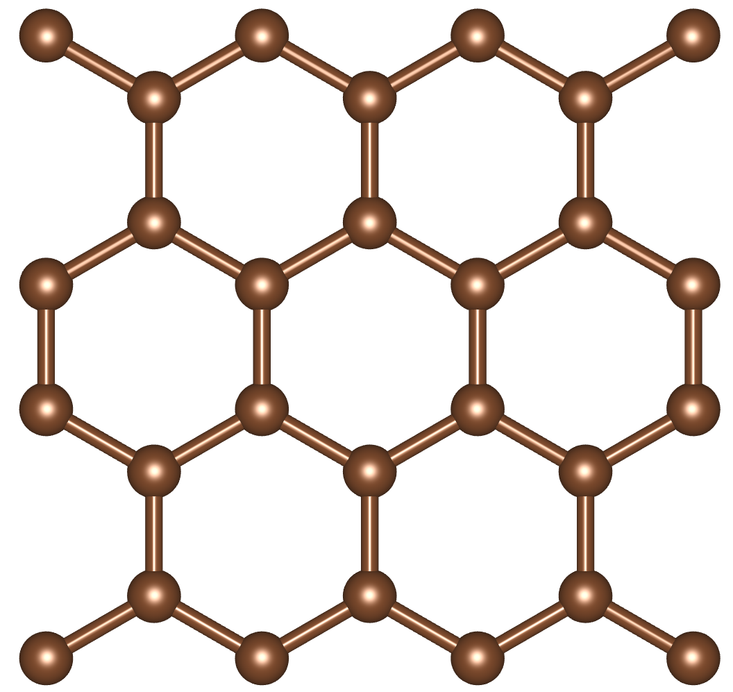
In this example (GR), how to optimize the cell parameter, how to calculate the band structure, and how to calculate density of states, are described.
Sample input file
nfinp_scf
WF_OPT    DAV
NTYP      1
NATM      2
TYPE      0
#NSPG     1017
GMAX      5.00
GMAXP    15.00
KPOINT_MESH   12  12  1
NSCF      400
WAY_MIX   3
MIX_ALPHA 0.4
SMEARING  MP
WIDTH     0.0010
EDELTA    0.1000D-11
NEG       24
CELL      4.6591  4.6591 18.89726878  90.00  90.00 120.00
&ATOMIC_SPECIES
 C  12.0107 pot.C_pbe3
&END
&ATOMIC_COORDINATES CRYSTAL
      0.00000000000      0.00000000000      0.00000000000    1    1    1
      0.33333333333      0.66666666667      0.00000000000    1    1    1
&END
Cell optimization
Go to the subdirectory Opt/ and as in the example of silicon, we manually change the in-plane lattice parameter (a and b) by 0.02 Bohr as
CELL 4.54 4.54 18.89726878 90.00 90.00 120.00
CELL 4.56 4.56 18.89726878 90.00 90.00 120.00
…
CELL 4.74 4.74 18.89726878 90.00 90.00 120.00
For each lattice constant we prepare an input file as nfinp_scf_a4.54, nfinp_scf_a4.56, … nfinp_scf_4.74 and execute STATE (min. and max. values, as well as the interval are arbitrary) by
$ qsub run.sh
Alternatively one can use run_multi.sh to automatically run a set of calculations.
We then plot the total energy as a function of lattice parameter (use getetot.sh in the same directory), and fit it to any function. In this example, let us use 6th order polynomial. The result looks like:
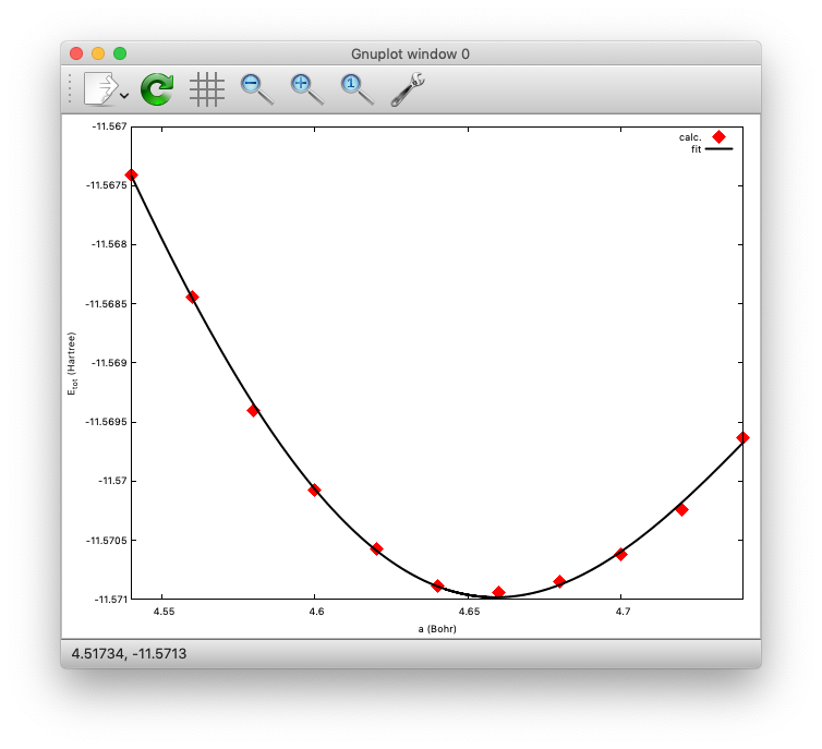
The minimum (equilibrium) can be found at a=4.6591 (Bohr). Compare with the experimental value.
Band structure calculation
We then use the theoretically optimized lattice parameter to calculate the band structure of graphene.
Change directory to Band/ and the files nfinp_scf and nfinp_band can be found.
To calculate the band structure, first we perform an SCF calculation to obtain a converged charge density (or potential) and perform a fixed charge (potential) non-SCF calculation for the high-symmetry k-points.
First perform the SCF calculation by using the following input file (nfinp_scf):
WF_OPT    DAV
NTYP      1
NATM      2
TYPE      0
#NSPG     1017
GMAX      5.00
GMAXP    15.00
KPOINT_MESH   12  12  1
NSCF      400
WAY_MIX   3
MIX_ALPHA 0.4
SMEARING  MP
WIDTH     0.0010
EDELTA    0.1000D-11
NEG       24
CELL      4.6591  4.6591 18.89726878  90.00  90.00 120.00
&ATOMIC_SPECIES
 C  12.0107 pot.C_pbe3
&END
&ATOMIC_COORDINATES CRYSTAL
      0.00000000000      0.00000000000      0.00000000000    1    1    1
      0.33333333333      0.66666666667      0.00000000000    1    1    1
&END
$ qsub run.sh
After converging the charge/potential, we perform the non-SCF band structure calculation by using the following input (nfinp_band):
TASK      BAND
WF_OPT    DAV
NTYP      1
NATM      2
TYPE      0
#NSPG     1017
GMAX      5.00
GMAXP    15.00
KPOINT_MESH   12  12  1
NSCF      400
WAY_MIX   3
MIX_WHAT  1
KBXMIX    20
MIX_ALPHA 0.4
SMEARING  MP
WIDTH     0.0010
EDELTA    0.1000D-11
NEG       24
CELL      4.6591  4.6591 18.89726878  90.00  90.00 120.00
&ATOMIC_SPECIES
 C  12.0107 pot.C_pbe3
&END
&ATOMIC_COORDINATES CRYSTAL
      0.00000000000      0.00000000000      0.00000000000    1    1    1
      0.33333333333      0.66666666667      0.00000000000    1    1    1
&END
&KPOINTS_BAND
 NKSEG 3
 KMESH 20 20 20
 KPOINTS
 0.00000000  0.00000000  0.00000000
 0.66666667 -0.33333333  0.00000000
 0.50000000  0.00000000  0.00000000
 0.00000000  0.00000000  0.00000000
&END
For the band structure calculation, we use the following keyword:
TASK BAND
To specify the high symmetry k-points, we add the following:
&KPOINTS_BAND
 NKSEG 3
 KMESH 20 20 20
 KPOINTS
 0.00000000  0.00000000  0.00000000
 0.66666667 -0.33333333  0.00000000
 0.50000000  0.00000000  0.00000000
 0.00000000  0.00000000  0.00000000
&END
Here we define the number of k-point segments by the keyword NKSEG:
NKSEG 3
k-point mesh for each segment:
KMESH 20 20 20
and NKSEG+1 k-points defining each segments:
KPOINTS
0.00000000  0.00000000  0.00000000
0.66666667 -0.33333333  0.00000000
0.50000000  0.00000000  0.00000000
0.00000000  0.00000000  0.00000000
Here the k-points are given in the unit of the reciprocal lattice vectors. To give the k-points in the cartesian coordinate, use:
KPOINTS CARTESIAN
Run the band structure calculation by replacing the input file with nfinp_band in run.sh
$ qsub run.sh
we obtain the file energy.data, which containg the Kohn-Sham eigenvalues, along with the k-points.
However, we cannot plot the band structure directory from energy.data and should be processed properly.
To convert the energy.data file into a plottable XY data, we use the energy2band program.
Type
$ energy2band
and you will be asked the numbers of bands considered, the number of bands to be plotted (can be the same as the previous one), the number of k-points considered (in this example, the eigenvalues at 61 k-points are calculated), and the energy origin (here, the Fermi level obtained in the SCF calculation will be used).
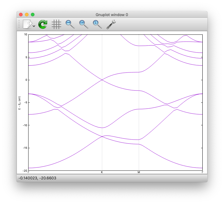
If the numbers are given properly, we obtain the file band.data, which can be used to plot the band directory by using gnuplot or grace.
Here is how the band structure looks like:
Density of states
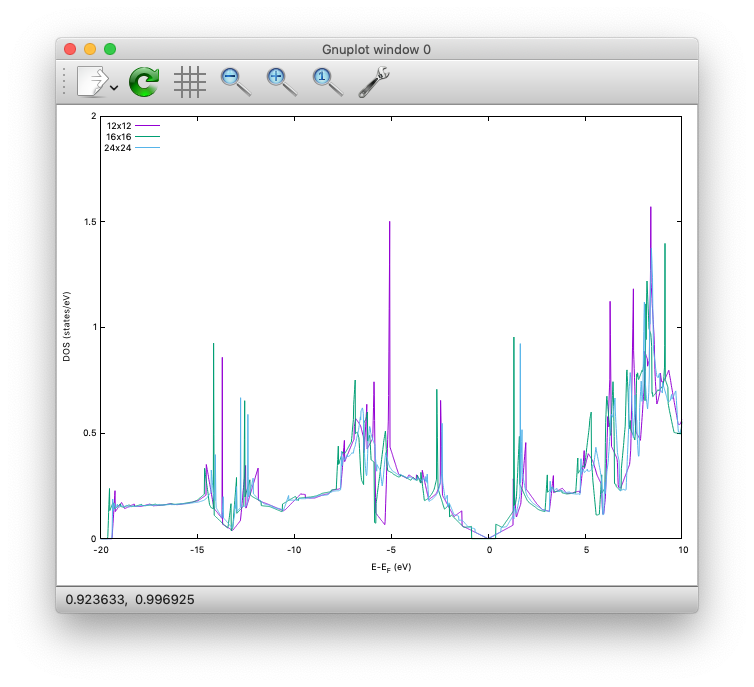
Now let us calculate the density of states (DOS) and projected DOS (PDOS) onto the atomic orbital.
Change the directory to DOS/ and we can find the directories 12x12/, 16x16/, and 24x24/, which indicate the k-point mesh used the calculation.
Let us change directory to 12x12 and have a look at the input file:
WF_OPT    DAV
NTYP      1
NATM      2
TYPE      0
#NSPG     1017
GMAX      5.00
GMAXP    15.00
KPOINT_MESH   12  12  1
NSCF      400
WAY_MIX   3
MIX_WHAT  1
KBXMIX    20
MIX_ALPHA 0.4
SMEARING  MP
WIDTH     0.0010
EDELTA    0.1000D-11
NEG       24
CELL      4.6591  4.6591 18.89726878  90.00  90.00 120.00
&ATOMIC_SPECIES
 C  12.0107 pot.C_pbe3
&END
&ATOMIC_COORDINATES CRYSTAL
      0.00000000000      0.00000000000      0.00000000000    1    1    1
      0.33333333333      0.66666666667      0.00000000000    1    1    1
&END
&DOS
 EMIN -20.0
 EMAX  10.0
&END
The total density of states is printed to dos.data, and the default energy window is from -0.5 to + 0.3 Hartree (-13.6057 to 8.1634 eV relative to the Fermi level).
To change the energy windown, we use the &DOS...&END block as:
&DOS
 EMIN -20.0
 EMAX  10.0
&END
where minimum and maximum energies are given in eV.
By Running the SCF calculation in each directory, we can observe the convergence of the density of states:
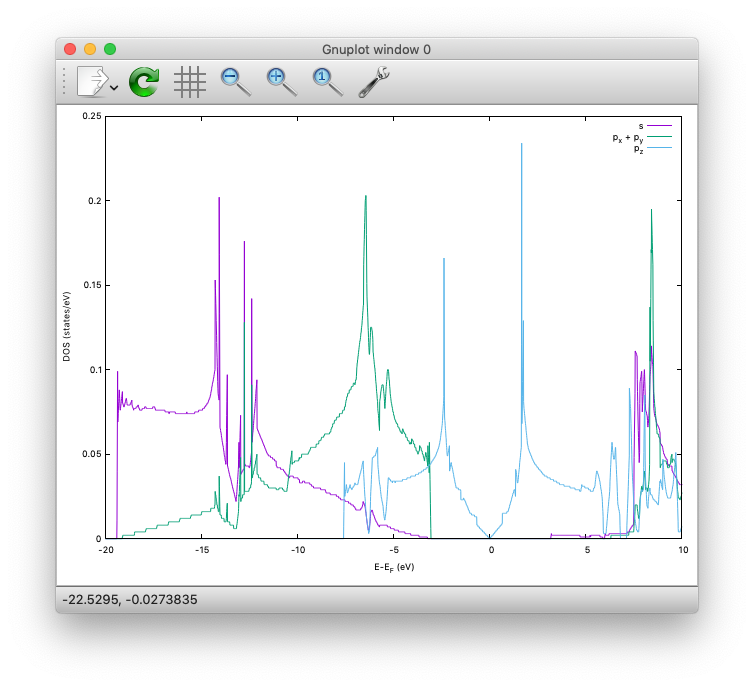
Finally, in the DOS/24x24 directory, we calculate PDOS.
The PDOS can be calculated at the end of the SCF calculation, or as a postprocess.
To compute PDOS in the SCF calculation, we can use the following nfinp_scf+pdos:
WF_OPT    DAV
NTYP      1
NATM      2
TYPE      0
#NSPG     1017
GMAX      5.00
GMAXP    15.00
KPOINT_MESH   24  24  1
NSCF      400
WAY_MIX   3
MIX_WHAT  1
KBXMIX    20
MIX_ALPHA 0.4
SMEARING  MP
WIDTH     0.0010
EDELTA    0.1000D-11
NEG       24
CELL      4.6591  4.6591 18.89726878  90.00  90.00 120.00
&ATOMIC_SPECIES
 C  12.0107 pot.C_pbe3
&END
&ATOMIC_COORDINATES CRYSTAL
      0.00000000000      0.00000000000      0.00000000000    1    1    1
      0.33333333333      0.66666666667      0.00000000000    1    1    1
&END
&PDOS
 NPDOSAO 1
 IPDOST  1
 EMIN    -20.00
 EMAX     10.00
 EWIDTH    0.10
 NPDOSE  3001
 RCUT    1.30
 RWIDTH  0.10
&END
where the block &PDOS...&END is added to set the parameters for the PDOS calculation:
&PDOS
 NPDOSAO 1
 IPDOST  1
 EMIN    -20.00
 EMAX     10.00
 EWIDTH    0.10
 NPDOSE  3001
 RCUT    1.30
 RWIDTH  0.10
&END
For the post-processing PDOS calculation, the following file (nfinp_pdos) can be used
TASK      PDOS
WF_OPT    DAV
NTYP      1
NATM      2
TYPE      0
#NSPG     1017
GMAX      5.00
GMAXP    15.00
KPOINT_MESH   24  24  1
NSCF      400
WAY_MIX   3
MIX_WHAT  1
KBXMIX    20
MIX_ALPHA 0.4
SMEARING  MP
WIDTH     0.0010
EDELTA    0.1000D-11
NEG       24
CELL      4.6591  4.6591 18.89726878  90.00  90.00 120.00
&ATOMIC_SPECIES
 C  12.0107 pot.C_pbe3
&END
&ATOMIC_COORDINATES CRYSTAL
      0.00000000000      0.00000000000      0.00000000000    1    1    1
      0.33333333333      0.66666666667      0.00000000000    1    1    1
&END
&PDOS
 NPDOSAO 1
 IPDOST  1
 EMIN    -20.00
 EMAX     10.00
 EWIDTH    0.10
 NPDOSE  3001
 RCUT    1.30
 RWIDTH  0.10
&END
where the keyword TASK is used to perfom the PDOS calculation:
TASK PDOS
In the &PDOS...&END block, number of atoms for which PDOSs are computed is defined by:
NPDOSAO 1
and corresponding atomic indices:
IPDOST 1
Number of IPDOST should equal to NPDOSAO.
Minimum and maximum energies (in eV) and number of grid points for the energy are defined by:
EMIN    -20.00
EMAX     10.00
NPDOSE  3001
and the smearing width (in eV) for the gaussian is defined by:
EWIDTH 0.10
We cutoff the atomic orbitals at certain radius RCUT (in Bohr):
RCUT 1.30
and the truncated orbital is smoothened by using the Fermi-Dirac type function with the width of RWIDTH:
RWIDTH 0.10
The number of RCUT and RWIDTH should corresponds to the number of atomic species (NTYPE).
The calculated PDOS for graphene can be visualized as:
Benzene
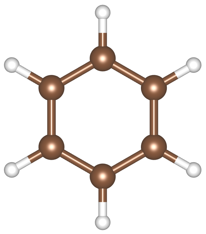
This example explain how to plot the molecular orbitals by using the benzene (C6H6) molecule.
The directory is C6H6/
SCF
Let us start with the SCF calculation by using the following input nfinp_scf:
WF_OPT DAV
NTYP   2
NATM   12
TYPE   0
GMAX    5.00
GMAXP  15.00
MIX_ALPHA 0.8
WIDTH   0.0010
EDELTA  0.1000D-08
NEG     24
CELL   15.00  15.00  15.00  90.00  90.00  90.00
&ATOMIC_SPECIES
 C  12.0107  pot.C_pbe3
 H   1.0079  pot.H_lda3
&END
&ATOMIC_COORDINATES XYZ
12
benzene example from https://openbabel.org/wiki/XYZ_(format)
  C        0.00000        1.40272        0.00000
  H        0.00000        2.49029        0.00000
  C       -1.21479        0.70136        0.00000
  H       -2.15666        1.24515        0.00000
  C       -1.21479       -0.70136        0.00000
  H       -2.15666       -1.24515        0.00000
  C        0.00000       -1.40272        0.00000
  H        0.00000       -2.49029        0.00000
  C        1.21479       -0.70136        0.00000
  H        2.15666       -1.24515        0.00000
  C        1.21479        0.70136        0.00000
  H        2.15666        1.24515        0.00000
&END
Here we show that the XYZ format can be used to give the atomic coordinates.
After the SCF is converged, wave functions in real space can be calculated by using nfinp_prtwfc:
TASK   PRTWFC
WF_OPT DAV
NTYP   2
NATM   12
TYPE   0
GMAX    5.00
GMAXP  15.00
MIX_ALPHA 0.8
WIDTH   0.0010
EDELTA  0.1000D-08
NEG     24
CELL   15.00  15.00  15.00  90.00  90.00  90.00
&ATOMIC_SPECIES
 C  12.0107  pot.C_pbe3
 H   1.0079  pot.H_lda3
&END
&ATOMIC_COORDINATES XYZ
12
benzene example from https://openbabel.org/wiki/XYZ_(format)
  C        0.00000        1.40272        0.00000
  H        0.00000        2.49029        0.00000
  C       -1.21479        0.70136        0.00000
  H       -2.15666        1.24515        0.00000
  C       -1.21479       -0.70136        0.00000
  H       -2.15666       -1.24515        0.00000
  C        0.00000       -1.40272        0.00000
  H        0.00000       -2.49029        0.00000
  C        1.21479       -0.70136        0.00000
  H        2.15666       -1.24515        0.00000
  C        1.21479        0.70136        0.00000
  H        2.15666        1.24515        0.00000
&END
&PLOT
 IKPT 1
 IBS  14
 IBE  17
 FORMAT XSF
&END
Wave function plot can be activated by setting:
TASK PRTWFC
and the k-points and range of bands of the wave functions to be plotted is given by the block:
&PLOT
 IKPT 1
 IBS  14
 IBE  17
 FORMAT XSF
&END
where IKPT is the index of the k-points, IBS and IBE are the indices of initial and final bands, respectively, and FORMAT is to specify the format of the output wave functions.
In this example, following files may be created:
nfwfn_kpt0001_band0014_re.xsf
nfwfn_kpt0001_band0014_im.xsf
nfwfn_kpt0001_band0015_re.xsf
nfwfn_kpt0001_band0015_im.xsf
nfwfn_kpt0001_band0016_re.xsf
nfwfn_kpt0001_band0016_im.xsf
nfwfn_kpt0001_band0017_re.xsf
nfwfn_kpt0001_band0017_im.xsf
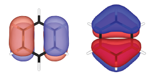
Real part (*_re*) and image part (*_im*) of the wave functions are generated separately. These wave functions can be plotted by using XCrySDen, VESTA, VMD, or alike. The real parts of the doubly degenerated highest occupied molecular orbitals (HOMOs) are visualized and shown below:
TiO2
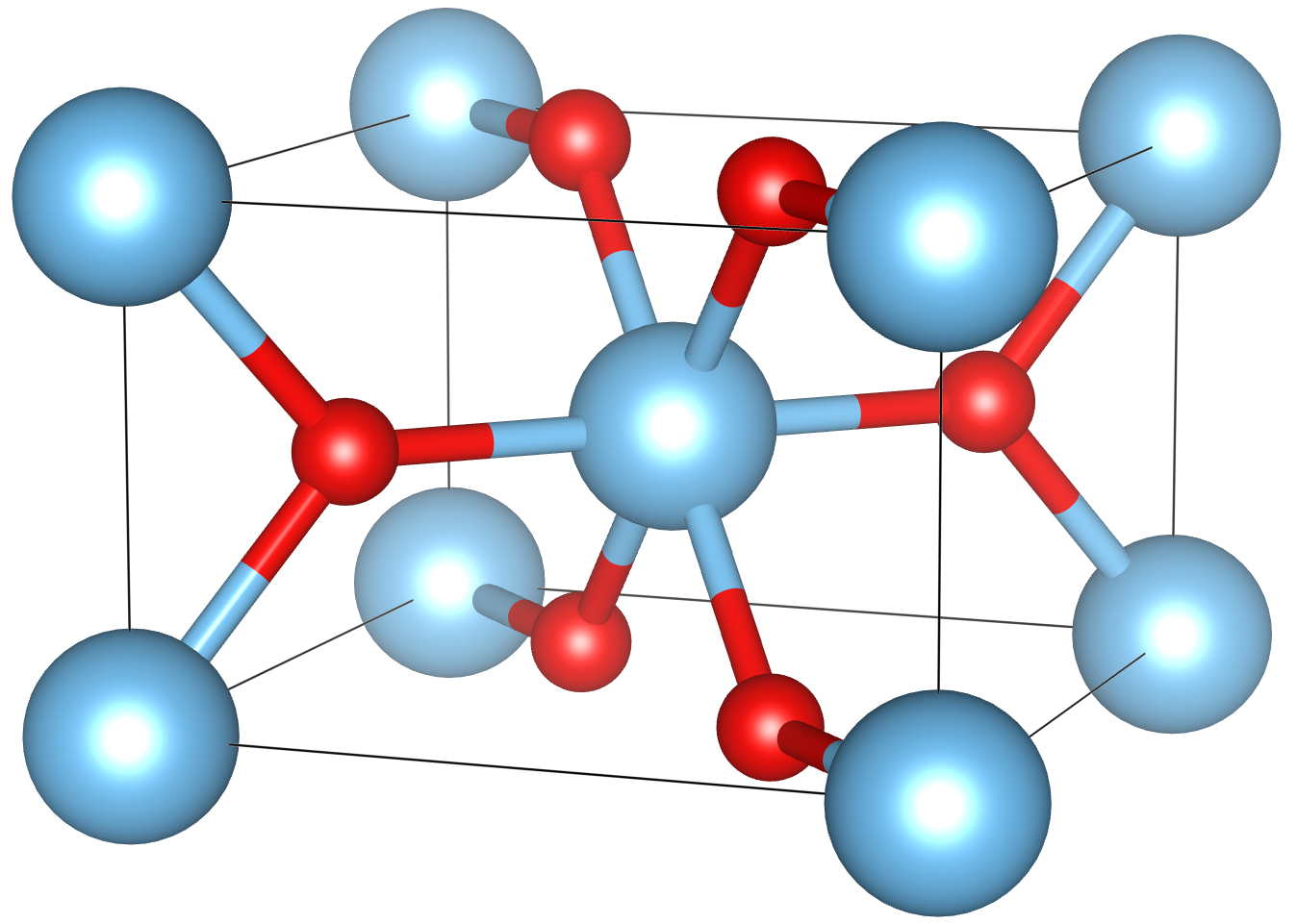
This example explains hot to perform a calculation with the on-site Coulomb potential correction (DFT+U) by using rutile.
Directory
TiO2/Input file for the DFT calculation
nfinp_scf
WF_OPT DAV
NTYP 2
NATM 6
TYPE 0
NSPG 136
GMAX    5.00
GMAXP  15.00
KPOINT_MESH    6  6  8
KPOINT_SHIFT   T  T  T
NSCF    200
KBXMIX 10
MIX_ALPHA 0.1
WIDTH   0.0002
EDELTA  0.1000D-09
NEG    30
CELL    8.68080000   8.68080000   5.58940000  90.00000000  90.00000000  90.00000000
XCTYPE  ldapw91
&ATOMIC_SPECIES
 Ti  47.947900 pot.Ti_pbe3
 O   15.994900 pot.O_pbe3
&END
&ATOMIC_COORDINATES CRYSTAL
      0.000000000000      0.000000000000      0.000000000000    1    0    1
      0.500000000000      0.500000000000      0.500000000000    1    0    1
      0.304829777700      0.304829777700      0.000000000000    1    1    2
      0.804829777700      0.195170222300      0.500000000000    1    1    2
     -0.304829777700     -0.304829777700      0.000000000000    1    1    2
     -0.804829777700     -0.195170222300      0.500000000000    1    1    2
&END
&HUBBARD
 NPROJ     2
 IPROJ     1    2
 HUBBARD_U 8.00 8.00
 RCUT      2.30 1.60
 RSMEAR    0.20 0.12
 NLMU      5
 LMU       5    6    7    8    9
&END
Note for this calculation, PW91 LDA (ldapw91) functional was used by setting:
XCTYPE ldapw91
For the on-site Coulomb potential (Hubbard U), the &HUBBARD...&END block is used:
&HUBBARD
 NPROJ     2
 IPROJ     1    2
 HUBBARD_U 8.00 8.00
 RCUT      2.30 1.60
 RSMEAR    0.20 0.12
 NLMU      5
 LMU       5    6    7    8    9
&END
Number of projectors are set by:
NPROJ 2
Indices for atoms on which the Hubbard U correction is applied:
IPROJ 1 2
Effective Hubbard U is defined by:
HUBBARD_U 8.00 8.00
Cutoff radii and smearing width for the localized orbitals are set by:
RCUT      2.30 1.60
RSMEAR    0.20 0.12
Number of the m components (usually 5 for the d state) is set by:
NLMU 5
and the indices for the m components are give by:
LMU 5 6 7 8 9
Compare the result (for instance, density of states written to dos.data) wihtout the Hubbard U correction.